Newtons Method
Extrapolation is the process of calculating the value of a function beyond the given range, while interpolation determines the value of a function for any intermediate value of the independent variable.
The general form of the newtons equaltion is
\( P_n(x)=f(x_0)+\sum_{k=1}^n \left( f(x_0, \dots , x_k) \cdot \prod_{i=0}^{k-1}{(x-x_i)} \right) \),
here n is the degree of the polynomial .
\( f(x_0, \dots , x_k) \) is the _k_th divided difference
it is defined as \( f(x_i, x_{i+1}, \dots , x_{i+k})=\frac{f(x_{i+1}, x_{i+2} \dots , x_{i+k}) – f(x_i, x_{i+1}, \dots , x_{i+k-1})}{x_{i+k}-x_i} \)
here the _k_th difference can also be defined as \( f(x_0, x_1, \dots , x_k)=\sum_{i=0}^k \left( \frac{f(x_i)}{ \prod_{j=0, j \neq i}^k (x_i-x_j) } \right) \)
Example : 1
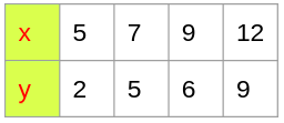
let us apply newtons equation for the above example.
\( P_n(x) = 2+\left(\frac{y_0}{x_0-x_1}+\frac{y_1}{x_1-x_0}\right)\left(x-x_0\right)+\left(\frac{y_1}{\left(x_0-x_1\right)\left(x_0-x_2\right)}+\frac{y_1}{\left(x_1-x_0\right)\left(x_1-x_2\right)}+\frac{y_2}{\left(x_2-x_0\right)\left(x_2-x_1\right)}\right)\left(\left(x-x_0\right)\left(x-x_1\right)\right)+\left(\frac{y_0}{\left(\left(x_0-x_1\right)\left(x_0-x_2\right)\right)\left(x_0-x_3\right)}+\frac{y_0}{\left(\left(x_1-x_0\right)\left(x_1-x_2\right)\right)\left(x_1-x_3\right)}+\frac{y_2}{\left(\left(9-5\right)\left(9-7\right)\right)\left(9-12\right)}+\frac{9}{\left(\left(12-5\right)\left(12-7\right)\right)\left(12-9\right)}\right)\left(\left(\left(x-5\right)\left(x-7\right)\right)\left(x-9\right)\right) \)
\( P_n(x) = 2+\left(\frac{2}{5-7}+\frac{5}{7-5}\right)\left(x-5\right)+\left(\frac{2}{\left(5-7\right)\left(5-9\right)}+\frac{5}{\left(7-5\right)\left(7-9\right)}+\frac{6}{\left(9-5\right)\left(9-7\right)}\right)\left(\left(x-5\right)\left(x-7\right)\right)+\left(\frac{2}{\left(\left(5-7\right)\left(5-9\right)\right)\left(5-12\right)}+\frac{5}{\left(\left(7-5\right)\left(7-9\right)\right)\left(7-12\right)}+\frac{6}{\left(\left(9-5\right)\left(9-7\right)\right)\left(9-12\right)}+\frac{9}{\left(\left(12-5\right)\left(12-7\right)\right)\left(12-9\right)}\right)\left(\left(\left(x-5\right)\left(x-7\right)\right)\left(x-9\right)\right) \)
\( f(x)=y_0 +(x-x_0) f[x_0, x_1]+(x-x_0)(x-x_1) f[x_0, x_1, x_2]+(x-x_0)(x-x_1)(x-x_2) f[x_0, x_1, x_2, x_3] \)
\( f(x)=2 + (x -5) * 1.5 + (x -5)(x -7) * -0.25 + (x -5)(x -7)(x -9) * 0.05 \)
\(f(x)=2 + (1.5x-7.5) + (-0.25x^2+3x-8.75) + (0.05x^3-1.05x^2+7.15x-15.75) \)
\(f(x)=0.05x^3-1.3x^2+11.65x-30 \)
now substitute \( x=10 \)
\( f(10)=0.05 * 10^3-1.3 * 10^2+11.65 * 10-30=6.5 \)
Now let us solve the above example by using s2
					%use s2
var data1 = SortedOrderedPairs(
                    doubleArrayOf(5.0,7.0,9.0,12.0), // x coordinates
                    doubleArrayOf (2.0,5.0,6.0,9.0)) // y coordinates
var np1: Interpolation = NewtonPolynomial()
var f1: UnivariateRealFunction = np1.fit(data1)
println(f1.evaluate(10.0))
Output : 6.5
					%use s2
// plotting the  above function using JGnuplot
val p = JGnuplot(false)
p.addPlot("x*x*x*0.05 - 1.3*x*x + 11.65*x -30 ")
p.plot()
Output :


Example : 2
Lorem ipsum dolor sit amet, consectetur adipiscing elit. Ut elit tellus, luctus nec ullamcorper mattis, pulvinar dapibus leo.

\( P_n(x) = 3+\left(\frac{3}{4-7}+\frac{5}{7-4}\right)\left(x-4\right)+\left(\frac{3}{\left(4-7\right)\left(4-15\right)}+\frac{5}{\left(7-4\right)\left(7-15\right)}+\frac{8}{\left(15-4\right)\left(15-7\right)}\right)\left(\left(x-4\right)\left(x-7\right)\right) \)
\(f(x)=3 + (x -4) xx 0.6667 + (x -4)(x -7) xx -0.0265 \)
\(f(x)=3 + (x-4) xx 0.6667 + (x^2-11x+28) xx -0.0265 \)
\(f(x)=3 + (0.6667x-2.6667) + (-0.0265x^2+0.2917x-0.7424) \)
\(f(x)=-0.0265x^2+0.9583x-0.4091 \)
Now substitute the value \( x=11 \)
\(f(11)=-0.0265 * 11^2+0.9583 * 11-0.4091= 6.924242424242424 \)
Now let us solve the above example on s2
					%use s2
var data1 = SortedOrderedPairs(
                    doubleArrayOf(4.0,7.0,15.0), // x coordinates
                    doubleArrayOf (3.0,5.0,8.0)) // y coordinates
var np1: Interpolation = NewtonPolynomial()
var f1: UnivariateRealFunction = np1.fit(data1)
println(f1.evaluate(11.0))
Output : 6.924242424242424
Plot :
					%use s2
// plot the above function by using JGnuplot
val p = JGnuplot(false)
p.addPlot("0.0265x^2+0.9583x-0.4091")
p.plot()
Output :

