
Introduction
Let us assume we have to find the answer to a question which is something like this: A car starts from rest and covers some distance in some seconds with constant acceleration. Find the acceleration of the car. In this scenario you have to deal with the speed of the car, distance, time taken, displacement, etc. equation of motion is required.
Classical mechanics is based on the Equations of Motion. For all macroscopic bodies moving at a speed considerably less than the speed of light, analysis of motion is done using Newton’s Equations of Motion. In this article, we will learn about these laws and their derivations along with the code in Kotlin S2.
Motion
First of all, let us know what motion actually is. As derived by the famous scientist Sir Isaac Newton we can define that motion as change in the position of an object with respect to time. That is, how much the object has moved in a time interval. We can represent the position using a reference point and then we can calculate the distance travelled by the object from that reference point. Similarly, we can calculate the time using a speed-watch which will represent the time taken for the change to happen.

Descriptions of motion
\(d\) is the distance.
\(s\) is displacement.
\(u\) is initial velocity.
\(v\) is final velocity.
\(a\) is acceleration.
\(t\) is the time taken for the motion to happen.
Distance
Distance is the actual measure of an object’s total change in position (over a period of time).

Note: Since distance is a scalar quantity hence it represents only the magnitude or the size or “how much”.
Displacement
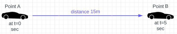
Displacement is defined as change in the position of an object(car). The arrow from point A to point B represents the change in the initial and final position of the object(car).

Note: Unlike distance, displacement is a vector quantity (an arrow) hence it represents both magnitude and direction, i.e., how much and which way.
Speed
Speed is a measure of how fast or slow an object(car) moves or changes its position. Speed is equal to the change in the distance covered by the object(car) per each unit of time. Mathematically speed is the ratio between the distance and time, i.e., distance divided by time.
\(v=\frac{\text{distance}}{\text{time}}\) i.e. \(v=\frac{d}{t}\)
The above graph gives us information about distance and time. By using the formula, we can calculate the speed. Let’s do it.
Question: If a car has traveled a total distance of 15m in 5 sec. calculate the speed.
\(\text{speed}=\frac{\text{distance}}{\text{time}}\) \(=\frac{15m}{5s}=3 m/s\).
Note: Speed is also a scalar quantity since both time and distance are scalar quantities too.
Velocity
Velocity can be defined as the rate of change of displacement of an object(car) per time unit, e.g., each second, each hour or each day. Mathematically this rate of change of position can represent as
\(\text{velocity}(v)=\frac{\text{displacement}}{\text{time}}\)
By looking at the above figure we get to know a couple of things like distance, displacement and time so by using the above formula we can easily calculate the velocity.
Question: If a car has covered 20m distance in 3 sec, calculate the velocity.
\(\text{velocity}(v)=\frac{\text{displacement}}{\text{time}}=\frac{15m}{3s}=5 m/s\).
Note: Velocity is vector quantity. It has information about both magnitude/size and direction.
Acceleration
Acceleration is the rate of change of the velocity of an object with respect to time. It is how much the velocity changes in a time unit. Acceleration is also a vector quantity and mathematically we can represent it as:
\(\text{acceleration}(a)=\frac{\text{velocity}(v)}{\text{time}(t)}\)
If the acceleration is negative, the object is slowing down. If the acceleration is positive, the object is speeding up. Watch out for the traffic police!
Equations of motion
The nature and the behavior of a physics system in terms of motion is determined by the equations of motion. There are three equations of motion.
\(v=u+at\),
\(s=u t+\frac{1}{2}at^{2}\),
\(v^{2}=u^{2}+2as\).
Derivation of the Equations of Motion by the Algebraic Method
Let’s see the derivations of the equations of motion by the algebraic method.
1st Equation of Motion
We all know that in general, acceleration is defined as the rate at which a body’s velocity changes over time. That is, how much the velocity changes in each unit of time. Mathematically, it is the difference in the final and initial velocities divided by the time taken for the change to happen.
\(\text{acceleration}(a)=\frac{(v-u)}{t}\).
where,
\(u\) = initial velocity
\(v\) = final velocity,
\(t\) = time taken
When we rearrange the above equation we get the following 1st equation of motion.
\(v=u+at\)2nd Equation of Motion
Imagine a body moving with an initial velocity of \(u\) under constant acceleration \(a\). The speed of the body becomes \(v\) after time \(t\) and the displacement becomes \(s\).
The velocity of an object is defined as the rate at which its displacement changes, or alternatively the displacement changes per unit of time. We can represent this mathematically as:
\(\text{velocity}=\frac{\text{distance}}{\text{time}}\).
After rearranging the terms, we get displacement \(s\), which is the product of the velocity and time period \(t\), when velocity \(v\) is constant.
\(\text{displacement} = \text{velocity} * \text{time}\).
If the velocity is not constant then we can use the average velocity in the place of velocity in the above equation, and rewrite the equation as follows:
\(\text{displacement} = \text{average velocity} * \text{time}\).
where,
\(\text{average velocity} = \frac{\text{final velocity}(v)+\text{initial velocity}(u)}{2}\),
\(s = \frac{u+(u+at)}{2} * t\),
\(s = \frac{(2u+at)}{2} * t\),
\(s = ut+\frac{1}{2}at^{2}\).
3rd Equation of Motion
As we know that the displacement is the rate of change of position of an object, i.e.,
\(\text{displacement} = \text{average velocity} * \text{time}\),
\(s = \frac{(u+v)}{2} * t\).
Now, from the 1st equation of motion, we know that
\(v=u + at\).
Rearranging the above formula,
we get
\(t = \frac{u-v}{a}\).
Now, substituting this value of \(t\) in the displacement formula we get the following equations.
\(s = \frac{(u+v)}{2} * \frac{v-u}{a}\),
\(2as=v^{2}-u^{2}\),
\(v^{2}=u^{2}+2as\).
Derivation of the Equations of Motion by the Calculus Method
Let’s demonstrate the derivations of the Equation of Motion by using the Calculus Method.
1st Equation of Motion
The acceleration of the object is constant so we use the definition of the instantaneous acceleration of the particle. That is, the acceleration of the object at a time point (rather than a time interval).
\(\text{instantaneous acceleration}(a)=\frac{dv}{dt}\).
Here, initial velocity = \(u\), the final velocity = \(v\), and the time interval \(dt\) is taken from \(t = o\) to \(t\) second.
The change in velocity \(dv\) is therefore the sum of all instantaneous acceleration \(a\) over all time points \(dt\). When \(a\) is a constant, it is simply
\(dv=a dt\).
By integrating both the sides, we get
\(\int_{v}^{u}dv=\int_{t}^{0}adt\),
\(v-u=a(t-0)\),
\(v=u+at\).
2nd Equation of Motion
Let’s use the 1st equation of motion:
\(v=u+at\).
Here the object is moving from time 0 to time t
\(v = \frac{ds}{dt} = u+at\),
\(ds = vdt = (u+at)dt\),
By integrating both sides, we get
\(\text{displacement}(s)=\int_{0}^{s}ds=\int_{0}^{t}vdt=\int_{0}^{t}(u+at)dt=ut+\frac{1}{2}at^{2}\).
3rd Equation of Motion
The average velocity for a constant accelerating object is given by:
\(\text{average velocity} = \frac{\text{final velocity}(v) + \text{initial velocity}(u)}{2}\).
Start with the first equation of motion:
\(v=u+ at\),
\(\text{time}(t)=\frac{(v-u)}{a}\),
\(\text{displacement}(s)= \text{average velocity} * \text{time taken}\),
\(s = \frac{(v+u)}{2} * \frac{(v-u)}{a} = \frac{(v^{2}-u^{2})}{2a}\),
\(v^{2}-u^{2} = 2aS\),
\(v^{2} = u^{2} + 2aS\),
Derivation of the Equations of Motion by the Graphical Method
Let’s now see the derivation of the equations of motion using the graphical method.

In the above velocity-time graph we can determine some details clearly.
- The velocity of the body increases from A to B in time t at a uniform rate.
- \(\bar{BC}\) is the final velocity and \(\bar{OC}\) is the total time t taken.
Initial velocity \(u = \bar{OA}\).
Final velocity \(v = \bar{BC}\).
1st Equation of Motion
From the graph we can see that
\(\bar{BC} = \bar{BD} + \bar{DC}\)Hence,
\(v = \bar{BD} + \bar{DC}\)\(v = \bar{BD} + \bar{OA}\) (because \(\bar{DC} = \bar{OA}\))
Then,
\(v = \bar{BD} + u\) (because \(\bar{OA} = u\)), equation (1)
Since the slope of a velocity-time graph is equal to acceleration \(a\).
We have,
\(a\) = slope of line \(\bar{AB}\)
\(a = \frac{\bar{BD}}{\bar{AD}}\)Since \(\bar{AD} = t\), the above equation becomes:
\(\bar{BD} = at\), equation (2)
Now, by combining both equations (1) and (2), we have
\(v = u + at\)2nd Equation of Motion
From the graph we can see that,
\(\text{distance traveled}(s)= \text{area of quadrilateral OABC} = \text{area of triangle ABD} + \text{area of rectangle OADC}\).
\(s=(\frac{1}{2} * \bar{AD} * \bar{BD}) + (\bar{OA} * \bar{OC})\).
As \(\bar{OA} = u\) and \(\bar{OC} = \bar{AD} = t\), the above equation becomes,
\(s = (\frac{1}{2} * t * \bar{BD})+ (u * t)\).
As \(\bar{BD} = at\) (from the graphical derivation of the 1st equation of motion), the equation becomes,
\(s = \frac{1}{2} * t * at + ut\).
On further simplification, the equation finally becomes
\(s = ut + \frac{1}{2}at^{2}\).
3rd Equation of Motion
The area of the quadrilateral can also be computed as follows.
\(s = \frac{1}{2} * \text{sum of the parallel sides} * \text{height}\),
\(s = \frac{1}{2} * (\bar{OA} + \bar{CB}) * \bar{OC}\).
Since \(\bar{OA} = u, \bar{CB} = v, \bar{OC} = t\),
The above equation transforms to
\(s = \frac{1}{2} * (v + u) * t\)Since \(t = \frac{(v – u)}{a}\),
The above equation can be represented as:
\(s = \frac{1}{2} * \frac{((v + u) * (v – u))}{a}\).
Rearranging the equation, we get
\(s = \frac{1}{2} * \frac{(v + u) * (v – u)}{a}\),
\(s = \frac{(v^{2} – u^{2})}{2a}\).
After rearranging we get the 3rd equation of motion.
\(v^{2} = u^{2} + 2as\).
Math Coding
Enough of theory, let’s now jump to some hands-on experiment with what we just learned. We will do the math coding of the equations of motion in S2.
// 1st equation of motion: final velocity
fun v(u : Double, a : Double, t : Double) : Double {
    var v = u + a * t;
    return v;
}

// compute the final velocity with inputs
// initial velocity = 5.0 m/s, acceleration = 2.0 m/s/s, time = 10 sec
val v = v(5.0, 2.0, 10.0)

// print out the final velocity
v
Here we set the initial velocity \(u = 5.0\) meters per second, acceleration \(a = 2.0\) meters per second per second and time \(t = 10.0\) seconds. The output is as follows:
25.0
We use two different ways to compute the displacement. We first use the second equation.
// 2nd equation of motion: displacement
fun s_1(u : Double, a : Double, t : Double) : Double {
    var s = u * t + 0.5 * a * t * t;
    return s;
}

// compute the displacement
// initial velocity = 5.0 m/s, acceleration = 2.0 m/s/s, time = 10 sec
val s_1 = s_1(5.0, 2.0, 10.0)

// print out the displacement
s_1
The output is as follows.
150.0
Alternatively, we can compute the displacement using the third equation of motion.
// 3rd equation of motion: displacement
// another formula to compute displacement
fun s_2(u : Double, a : Double, t : Double) : Double {
    var s = (v*v - u*u) / 2.0 / a;
    return s;
}

// compute the displacement
// initial velocity = 5.0 m/s, acceleration = 2.0 m/s/s, time = 10 sec
val s_2 = s_2(5.0, 2.0, 10.0)

// print out the displacement
s_2
The output is as follows.
150.0
We can also use the third equation of motion to compute the final velocity. We need to compute the square of velocity first.
// 3rd equation of motion: velocity squared
fun v2(u : Double, a : Double, s : Double) : Double {
    var v2 = u*u + 2.0 * a * s;
    return v2;
}

// compute the square of the final velocity
// initial velocity = 5.0 m/s, acceleration = 2.0 m/s/s, displacement = 150 m
val v2 = v2(5.0, 2.0, 150.0)

// print out the velocity squared
v2
The output is as follows.
625.0
The final velocity is the square root of the last result.
// print out the final velocity
sqrt(v2)
25.0
As expected, it is the same as what we input for the first two equations.
Try out the equations with your own input and numbers. Play with the code to see what you get. It is fun to do experiments! Let us what you think and leave us comments below.
The source code can be found in our GitHub:
https://github.com/nmltd/s2-public/blob/main/Blogs/equations_of_motion.ipynb
Alternatively, you can run the code on S2:
https://s21.nm.dev/hub/user-redirect/lab/tree/s2-public/Blogs/equations_of_motion.ipynb

Conclusion
It is important to note that we have derived the set of equations of motion without doing experiments or data. We construct a theory entirely out of imagination. The concept of space (position) and time are intuitive. We can measure them using a ruler and a clock. While the concept of speed may be familiar by daily experience, the concept of acceleration is a pure theoretical construct. By introducing or inventing the “new” notion of acceleration, we construct a theory of motion, and tie together all fundamental quantities, namely, space, time, and velocity, using precise mathematical equations. This illustrates how we can invent new physics theory using pure imagination. This is true for our simple framework of motion but it is also true for much more advanced theories like the Special Relativity. Both Newton and Einstein constructed their ground breaking theories by inventing new concepts by pure imagination without actually doing any experiments or data. They then expressed their concepts precisely using mathematics.
No comment yet, add your voice below!