Introduction

Probability Distribution of Random Variable is one of the foundational pillars of machine learning since it deals with the study of random phenomena. Despite its enormous size, though, it is easy to get lost, especially for those who are self-taught.

We will discuss some fundamentals in the following sections, including random variables and probability distributions, which are especially relevant to machine learning.

To understand why those concepts are important to understand, let us first think about why we should care about them in the first place.

What is probability?Why understand it?

Because of incomplete observability, machine learning is often associated with uncertainty and stochastic quantities – hence, probably with sampled data.

In spite of the fact that we have little data and don’t know the entire population, we want to make reliable conclusions about the behavior of a random variable.

The sampled data can be generalized to the population, so we must estimate the real underlying data-generation process.


We can compute the probability of a particular outcome by accounting for the results’ variability by understanding the probability distribution. It allows us to generalize from samples to populations, to estimate the function that generates data, and to predict more accurately the behavior of random variables.

Introduction to the Random Variable

Random variables are variables whose values depend on the outcome of a random event. Alternatively, it can be referred to as a function mapping from the sample space to the measurable space 

Let’s assume we have four students [A, B, C, D] in our sample space. When we pick a random student A and measure his height in centimeters, we can think of the random variable (H) as a function with input student and output height as a real number.

H(student)=height

The following is an example of how we can visualize this small example.


Depending on the outcome – which student is selected at random – our random variable (H) can take on different characteristics, or different values when it comes to height in centimeters

There are two types of random variables: discrete and continuous

Random variables are considered discrete when there are only a finite or countably infinite number of possible values. There are various discrete random variables, including the number of students in a classroom, the number of correct answers to a test, and the number of children in a family.

In contrast, random variable is continuous if the number of valid values between any two values is infinite. Continuous random variables include pressure, height, mass, and distance.

Probability distributions allow us to answer the following question: What is the likelihood of our random variable taking a particular state? Or put another way, what is the probability?

Probability Distribution

A probability distribution describes the likelihood that a random variable will take one of its possible states. An experiment’s probability distribution, then, is a mathematical function that determines the odds of different outcomes.

The function of it is more generally described as

P: A –>R

The probability is the mapping of the input space A referred to as a sample space – to a real number.

A probability distribution described by the above function must follow the Kolmogorov axioms:

  1. Non-negativity
  2. No probability exceeds 1
  3. Additivity of any countable disjoint (mutually exclusive) events

There is a difference between describing a probability distribution using a probability mass or density function based on whether the random variable is discrete or continuous.

Probability Mass Function

PMFs are used to describe the distribution of probability over discrete random variables. 

The function indicates how likely it is that a random variable will be exactly equal to a specific value.

All probabilities for each state are added together to equal one, and the sum for each state lies in the range [0, 1].

As an example, let’s imagine a plot whose x-axis represents states and y-axis represents probability of each state. Imagine the probability or the PMF as a barplot stacked on top of a state if we approach the problem this way.

Discrete probability distributions consist of three main types: Bernoulli, binomial and geometric.


Bernoulli Distribution

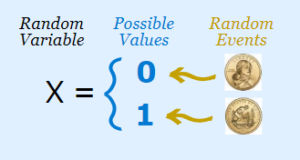
A Bernoulli distribution is a discrete probability distribution for the value of a binary random variable, which has either a value of 1 or 0. It is named after Swiss mathematician Jacob Bernoulli.

It can be thought of as a model that provides the set of possible outcomes for a single experiment, and it can be answered with a simple yes or no question.

In more formal terms, this function is expressed by the following equation


This equation essentially evaluates to p if k=1 or to (1-p) if k=0. There is only one parameter associated with the Bernoulli distribution, p.

Consider tossing a fair coin once. A probability of getting heads of coin is equal to 0.5. We see the following plot when visualizing the PMF:


Binomial Distribution

In a series of n independent trials, each with a binary result, a binomial distribution describes the discrete probability distribution of the number of successes. The likelihood of success or failure is expressed by probability p or (1-p).

In this way, we can parametrize the binomial distribution by the parameters

n∈ N , p ∈ [0,1] 

To express a binomial distribution with more formal terms, we can use the following equation:

Success of k is determined by p to the power of k, whereas failure is determined by (1-p) to the power of n minus k, which is simply the number of trials minus the one during which we obtain k.

We have “n choose k” ways to distribute the success k in n trials since success can occur anywhere in n trials.

Take our coin-tossing example from before as an example and let’s expand on it.

To begin, we’ll flip the fair coin three times, while keeping an eye on the random variable that describes the number of heads that are obtained.

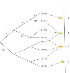
We can simply use the equation from before in order to compute the probability of the coin coming up head twice.


This results in a probability P(2) = 0.375. We obtain the following distribution if we follow the same process for the remaining probabilities:

Geometric Distribution

Let’s say we want to know how many times we have to flip a coin until it comes up heads for the first time.

With n independent trials and a probability of p, the geometric distribution gives the probability that the first successful trial will occur.

This can be stated in more formal terms as follows:

Based on the number of trials required up to and including success, one can calculate the probability of a success event.

In order to calculate the geometric distribution, we need to make the following assumptions:

  1. Independence
  2. Only two outcomes are possible for each trial
  3. Trials are all equal in terms of success probability

Consider the probability of the coin coming up heads for the first time when answering the question of the number of trials needed.

Probability Density Function

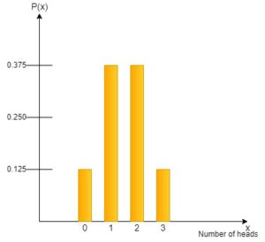
As you learned in the earlier sections, random variables are either discrete or continuous. A probability mass function can be used to describe the probability distribution if it is discrete.

As we are dealing with continuous variables, a probability density function (PDF) is appropriate for describing the probability distribution.

PDFs do not directly indicate the probability of a random variable taking a specific state, as the PMF does. Rather, it represents the probability of landing within an infinitesimal area. Another way to put it is the PDF indicates the likelihood of a random variable lying between a certain range of values.

In order to determine the actual probability mass, we must integrate, which yields the area above the x-axis but beneath the density function.


There must be no negative values in the probability density function and the integral should be 1.


In probability theory, the gaussian distribution or normal distribution is one of the most common continuous distributions.

Gaussian Distribution

In situations where a real-valued random variable whose distribution is unknown, the Gaussian distribution is often considered a reasonable choice.

There is a main reason for this due to the central limit theorem, which states that the average of many independent random variables with finite mean and variance can be seen as a random variable in itself – one with a normal distribution as the number of observations increases.

The advantage of this is that complex systems can be modeled as Gaussian distributed even when their individual components have more complex structural characteristics or distributions.

This is also due to the fact that it inserts the least amount of prior knowledge into the equation when modeling a continuous variable.

Gaussian distribution is expressed formally as


Here the parameter  µ represents the mean, whileσ²describes the variance.

A bell-shaped distribution’s peak will be defined by its mean, while its width will be determined by its variance or standard deviation.

Normal distributions are illustrated as follows:


Let us understand more about the concept of Probability Distribution with an example

A coin is tossed three times. Will make the following assumptions: X = the number of heads, Y = the number of headruns. (A ‘head run’ occurs when at least two heads occur consecutively.) Calculate the probability function for X and Y.

Answered : The possible outcomes of the experiment are S = {HHH, HHT, HTH, HTT, THH, THT, TTH, TTT}. “X” refers to the number of heads. Among the possible numbers are 0, 1, 2, and 3.

Coding part

Lets demonstrate a simple example of distribution of random variable in kotlin S2.

 import statements has been entered and class has been created for generating number for further use.

				
					import java.util.HashMap // implement the map interface and thus stores key values pairs
// class for generating the random numbers
class numbergenerated {
     val distribution: MutableMap? // double and int variables are declared for distribution
     var distSum = 0.0 // variables are being assigned 


In this block we have created a function which takes care of generating numbers with the help of class and with that test process is also going on to validate those numbers to get random numbers.

				
					// function is created to add numbers 
    fun main() {
        val number = numbergenerated() // class is being reused here
        number.addNumber(1, 0.2)
        number.addNumber(2, 0.3)
        number.addNumber(3, 0.5)
        val testCount = 1000000 // counting....
        val test = HashMap()
        for (i in 0 until testCount) {
            val random = number.getDistributedRandomNumber()!!//variable for random numbers
            test[random] = if (test[random] == null) 1.0 / testCount else test[random]!! + 1.0 / testCount
        } // random numbers get tested to see of they are null or not with condition statement
        println(test.toString()) // printing the result of test
    }


Init statement is called for initializing the distribution as key value pairs with help of hashmap. Further we have also did the similar approach to find the new random value number.

				
					 init {
        distribution = HashMap()
    }
// similarly here for distribution of random variables 
    fun addNumber(value: Int, distribution: Double) {
        if (this.distribution?.get(value) != null) {
            distSum -= this.distribution.get(value)!!
        }
        this.distribution?.set(value, distribution)
        distSum += distribution
    }


Here we are fetching those random numbers and trying to get the ratio and distribution with respect to and finally return the value generated

				
					// to get the random values of distributed varible 
    fun getDistributedRandomNumber(): Int? {
        val rand = Math.random()
        val ratio = 1.0f / distSum
        var tempDist = 0.0
        for (i in distribution?.keys!!) {
            tempDist += distribution.get(i)!!
            if (rand / ratio <= tempDist) {
                return i
            }
        }
        return 0
    }
}


Finally we have reached to the point where we get the final random value generated .


					val a = DistributedRandomNumberGenerator() // varible for getting the final value
a.main()


Ouptut

Run this code again and again to get the different random variable each time.

Thank You for your time. Have a good day.