Geometric intuition behind LR
Logistic regression is very geometrically elegant algorithm. It comes under supervised learning. Even though the name has regression in it, it is actually a classification technique. It predicts the categorical dependent variable using a set of independent variables. The decision surface in logistic regression is line or a plane.

As we can see our data is linearly separable. Linearly separable means, a line or a plane that seperate positive class and negative class.

So the next question is, how do you represent a plane or a line? Plane is represented in two parts, (W,b) W is normal to the plane and b is intercept. So the equation of a plane or line in n-dim space is given as wT*x + b =0(w transpose * x +b=0). If plane π passes through the origin then value of b is 0 so eq becomes wTx = 0 Big assumption that logistic regression makes is, it assumes that the classes are perfectly separable or almost perfectly separable.
Task in logistic regression is to find w and b, if we find the value of w and b we can get the plane

Now lets take two points xi and xj and it’s distance di and dj from the plane, for simplicity let’s assume that plane is passing through the origin. Since w and xi are on the same side of the plane distance di will be greater than 0 (di=wTxi > 0) and w and xj are on opposite side of the plane, distance dj will be less than 0(dj=wTxj < 0)
So intuitively, what classifier does is, it predicts the value of w in the equation, if wTxi > 0 then its class label yi will be +1 and if wTxj < 0 then its class label yj will be -1.


Case 1:
When the classifier wTx has value greater than 0 and class label yi is a positive point(+1), so when we product them (y*wTx) its result will be greater than 0, and we can conclude that it correctly classified the point.
Case 2:
When the classifier wTx has value less than 0 and class label yi is a negative point(-1), so when we product them (y*wTx) its result will be greater than 0, and we can conclude that it correctly classified the point.
Case 3:
When the classifier wTx has value less than 0 and class label yi is a positive point(+1), so when we product them (y*wTx) its result will be lesser than 0, and we can conclude that it incorrectly classified the point.
Case 4:
When the classifier wTx has value greater than 0 and class label yi is a negative point(-1), so when we product them (y*wTx) its result will be lesser than 0, and we can conclude that it incorrectly classified the point.
Classifier would be proven good if and only if there are minimum number of misclassified points or maximum number of correctly classified points
Mathematically speaking, imagine we have n-datapoints, so we have to maximize yi*wT*x. Mathematically written as MAX Σ yi*wT*xi. If you look carefully xi and yi are part of the dataset, so we can’t manipulate it, so we have to change or vary ‘w’ so formula becomes MAX(w) Σ yi*wT*xi So as we change w, equation will change and we want to find such w that maximizes the equation. So in a nutshell we want to find the optimal w, let’s call it w*, such that it maximizes the equation.
Equation can be written as w*=argmax(w)Σ yi*wT*xi. argmax states, whichever w maximizes the sum call it w*
This above equation is an optimization problem, when we solve this optimization problem we will get the optimal w*, hence giving us a good classifier.
The term yi*wT*xi in the equation w*=argmax(w)Σ yi*wT*xi is known as signed distance, signed distance intutively means distance of a given point from the plane.
Squashing and sigmoid

Let’s discuss is logistic regression prone to outlier or not.
Case 1
In the given example, let’s assume π1 be the plane that seperate the points. Just for simplicity let the distance between positive points and plane be +1 and distance between negative points and plane be -1. And there exist a negative point on the positive side of the plane with a distance of 100 as an outlier. As we know the value given by formula for correctly classified point is positive and for incorrectly classified point is negative. So the resulting value for the case 1 using signed distance formula(Σyi*wT*xi) would 1+1+1+1+1+1+1+1-100 = – 92

Case 2
In the given example, let’s assume π2 be the plane that seperate the points. Just for simplicity let the distance between each consecutive positive points and negative points be +1 and -1. And the distance between the plane and the outlier point be +1. As we know the value given by formula for correctly classified point is positive and for incorrectly classified point is negative. Over here as negative points are classified as positive points they will hold negative value for signed distance. So the resulting value for the case 2 using signed distance formula(Σyi*wT*xi) would 1+2+3+4-1-1-3-4+1= + 1
Argmax will choose plane π2 over π1, as π2 > π1, even though π1 is performing better with just 1 mis-classified point. One single extreme outlier point is changing the model that is very bad. Which means max sum of signed distance is not prone to outlier, so we need to modify this equation to make it less prone to outlier.
One of such technique is called as SQUASHING. Idea behind squashing is, instead of using simple signed distance we will modify the equation such that, if the signed distance is small, keep it as it is, if signed distance is large make it a smaller value.
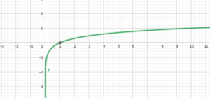
In a nutshell, we want to come up with the function such that, when signed distance is small it will grow smoothly and as soon as signed distance starts to increase it will taper off, such that maximum value will never be more than something. Intuitively it means, w*=argmax(w) Σ f(y*wT*x). As you can see below green line represents the function, as distance is small it behaves as a linear function, it starts to taper off as the distance increases.

One such function is SIGMOID(σ). Formula for sigmoid function is 1/1+exp-x it has max value of 1 and min value of 0.

There exist many such function, but why sigmoid function?? because it has very nice probabilistic interpretation and sigmoid function is easy to differentiate (we need a fucntion that is easy to differentiate for optimization, as it is a tedious task)
Probablistic interpretation here means, assume there is a data point on the plane, so the distance will be 0, so sigmoid function for 0 is 0.5 as you can see in above graph. If the distance is less than 0 value would be less than 0.5 and if the distance is greater than 0, it would be more than 0.5
Therefore we need to optimize, max sum of transformed sigmoid function, w*=argmax(w) Σ σ(yi*wT*xi) or w*=argmax(w) Σ 1/(1+ exp (-yi*wT*xi)) as formula for sigmoid is 1/1+exp^-x.
Formulation for objective function
MONOTONIC FUNCTION
If x increases and g(x) also increases such a function is called monotonically increasing function. More mathematically speaking, if x1 > x2 then g(x1) > g(x2) then g(x) is said to be monotonically increasing function.
Log(x) is monotonically increasing function, as you can observe below.

Imagine i have an optimization problem as x*=argmin(x) x2
Plot x2 look like parabola, and the minimum value of this function is 0 . So answer for x* is 0
x2 is monotonically increasing when x > 0
x2 is monotonically decreasing when x < 0

Let’s assume i define a function called g(x)= log(x).
Our initial optimization problem was x*=argmin(x)f(x) where f(x) = x2
What if we do x’ =argmin(x) g(f(x))
Intutively what i am saying is x’= =argmin(x) log( x2 )
we can claim x*= x’ because g(x) is monotonic function. Graphically speaking, if we observe minimum of x2 occurs at 0, and minimum of log(x2) also occurs at 0
There is a rigouros proof in theory of optimization that if g(x) is monotonic function then argmin(x)f(x)=argmin(x)g(f(x)) argmax(x)f(x)=argmax(x)g(f(x))
Now coming back to our orignal problem which is w*=argmax(w) Σ 1/(1+ exp (-yi*wT*xi))
So if we use g(x) as log(x) which is a monotonic function.
We can say, w* = argmax(w) Σ log(1/(1+ exp (-yi*wT*xi))) where 1/(1+ exp (-yi*wT*xi)) is f(x)
And as we know log(1/x)= – log(x)
w* = argmax(w) Σ -log((1+ exp (-yi*wT*xi)))
Now mathematically max(f(x)) = min(-f(x))
So our modified optimization problem is w* = argmin(w) Σ log((1+ exp (-yi*wT*xi)))
This was our geometric intution behind logistic regression.
Probabilistic Interpretation for LR is w* = argmin(w) Σ -yi log pi – (1-yi) log(1-pi) where pi= σ(wTxi)
Both equation are one and the same, There is beautiful in depth proof of probablistic interpretation in this link https://www.cs.cmu.edu/~tom/mlbook/NBayesLogReg.pdf
Getting hands-on
We will be using Weka, an open source software to get hands-on experience of logistic regression. Before diving into code let’s understand what is weka. Weka is a collection of machine learning algorithms for data mining tasks. It contains tools for data preparation, classification, regression, clustering. Math over here would be taken care by WEKA. This is where you will learn more about it. https://www.cs.waikato.ac.nz/ml/weka/
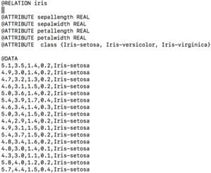
File format: We will be using ARFF file format as data for classification task. So what is an ARFF file format? An ARFF (Attribute-Relation File Format) file is an ASCII text file that describes a list of instances sharing a set of attributes. It has 2 sections, 1) Header information: which contains name of relation, list of attributes and it’s type. 2) Data information: contains the data. Below is the example of how ARFF files look like.
(Installing weka on your local system could be a tedious task. So on our S2 platform we have already installed it, you just have to use it with one magic command i.e %use weka)
Let's get started
For every machine learning problem first step is to aquire data, so we will be using weka dataset available here https://storm.cis.fordham.edu/~gweiss/data-mining/datasets.html
We would be using weather.nominal data for this tutorial. Make sure you create your own custom test data(just mix match some combination to check does our model works terrible or amazing)


Let’s dive into coding part
Import this required libarary which will be used further.
Logistic: Algorithm for logistic regression.
ConverterUtils: Simple Utility program for converter packages.
					//importing the required library
import weka.classifiers.functions.Logistic
import weka.core.converters.ConverterUtils
We have acquired the data, so now let’s load the data into memory.
ConverterUtils.DataSource: Helper class to load data from files, using converterutils class, it determines which converter to use for loading the data into memory.
					val source = ConverterUtils.DataSource("weather.nominal.arff")
val traindataset = source.dataSet
Further step is to tell our data to seperate variable and class that we want to predict.
[ setClassIndex(traindataset.numAttributes() – 1) ] indicates that, from my training data, last attribute should be considered as class label. And to get number of classes we will use numClasses().
					traindataset.setClassIndex(traindataset.numAttributes() - 1)
val numClasses = traindataset.numClasses()
So our class labels are “yes” and “No”. Our model should understand class-label, so instead of passing yes and no to the classifier we will pass distinct value.
					for (i in 0 until numClasses) {
    val classvalue = traindataset.classAttribute().value(i)
    println("Class Value " + i + " is " + classvalue)
}

Finally our data is ready to be passed to the classifier for building model with less than 3 lines of code.
					val log = Logistic()
log.buildClassifier(traindataset)
So our model is ready, let’s get our test data ready using exact same step that we did for training data.
					val source1 = ConverterUtils.DataSource("weather.nominal .test.arff")
val testdataset = source1.dataSet
testdataset.setClassIndex(testdataset.numAttributes() - 1)
Next we will use our classifier to make predictions on test data
					println("Actual, pred")
//num instance returns no. of instance of the dataset
for (i in 0 until testdataset.numInstances())
{
    //Converting actual class value of test data to distinct value
    val actualclass = testdataset.instance(i).classValue()
    val actual = testdataset.classAttribute().value(actualclass.toInt())

    //Using our classifier to predict test data class label and compare it with actual values
    val newinst = testdataset.instance(i)

    //classify the given test instance
    val pred = log.classifyInstance(newinst)
    val predstring = testdataset.classAttribute().value(pred.toInt())
    // comparison of predicted and actual

    println("$actual,$predstring")
}

As we can see we correctly classified 5 instance from 6, resulting in 83.33 % accuracy.
Let’s evaluate our machine learning model and have some statistical insight on it.
Kappa statistic: Use to check reliability of inter-rater items.
Mean absolute error: Use as an error measure between observation.
Root mean squared error: Use to check difference between value predicted by model.
Relative absolute error: Expressed as ratio comparing mean error and error made by model.
Root relative squared error: What should be the value if simple predictor was used.
					val eval = weka.classifiers.Evaluation(traindataset)
eval.evaluateModel(log, testdataset)
print(eval.toSummaryString("\nResults\n======\n", false))

We now conclude the topic, “Unraveling Logistic Regression”.
Thank you for spending time on this course! Hope you learned a lot.