Let us first look into the basics:
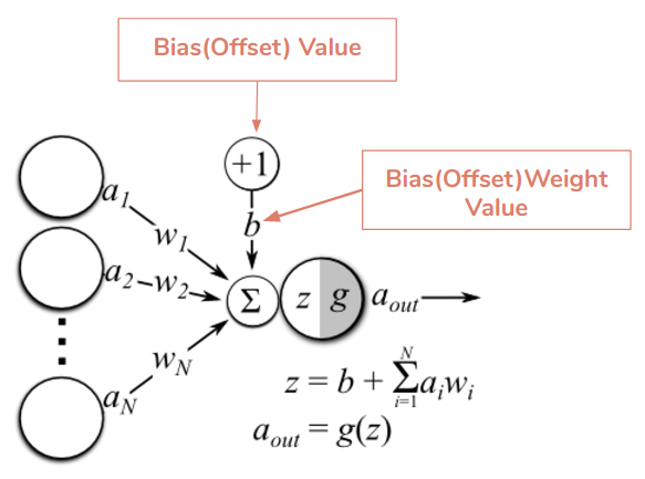
Weights and biases (commonly referred to as w and b) are the learnable parameters of deep learning models, including neural networks. Neurons are the basic units of a neural network. In an ANN, each neuron in a layer is connected to some or all of the neurons in the next layer. When the inputs are transmitted between neurons, the weights are applied to the inputs along with the bias.
Weights control the signal (or the strength of the connection) between two neurons. In other words, a weight decides how much influence the input will have on the output. Biases, which are constant, are an additional input into the next layer that will always have the value of 1. Bias units are not influenced by the previous layer (they do not have any incoming connections) but they do have outgoing connections with their own weights. The bias unit guarantees that even when all the inputs are zeros there will still be an activation in the neuron.
The importance of effective weight initialization:
To build a machine learning algorithm, usually we define an architecture (e.g. Logistic regression, Support Vector Machine, Neural Network) and train it to learn parameters. The common training process for neural networks can be listed as:
Initialization of Neural Network: Initialize weights and biases.
Forward propagation: Using the given input X, weights W, and biases b, for every layer we compute a linear combination of inputs and weights (Z) and then apply activation function to linear combination (A). At the final layer (l), we compute f(A(l-1)) which could be a sigmoid (for binary classification problem), softmax (for multi-class classification problem), and this gives the final prediction.
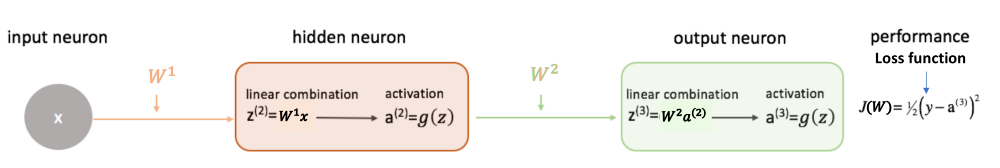
Compute the loss function: The loss function includes both the actual label (y) and predicted label (y_hat) in its expression. It shows how far our predictions are from the actual target, and our main objective is to minimize the loss function.
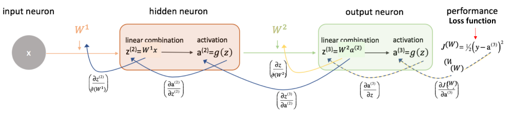
Backward Propagation: In backpropagation, we find the gradients of the loss function, which is a function of y and y_hat, and gradients wrt A, W, and b called dA, dW, and db. By using these gradients, we update the values of the parameters from the last layer to the first layer.
Repeat the above 3 steps for n epochs till we observe that the loss function is minimized.
Now, given a new data point, you can use the model to predict its class. The initialization step can be critical to the model’s ultimate performance, and it requires the right method.
Deep learning based architectures are characterized by many hidden layers of neurons. However, the main limitation of these architectures is the long time required for training. Obtaining excellent accuracy and reasonable training time is a challenging objective for the deep learning community. Selecting an appropriate weight initialization strategy is critical when training different neural networks. Weight initialization represents the manner of setting initial weight values of a neural network layer. Deep learning methods are very sensitive to the values of initial weights. Initialization of weight seeks to assist in establishing a stable neural network learning bias and shorten convergence time.
The figure below shows the weight matrix showing the weights in different layers of a neural network:
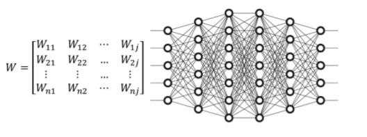
The goal of weight initialization is to prevent layer activation outputs from exploding or vanishing during the training of neural network. Training the network without a useful weight initialization can lead to a very slow convergence or an inability to converge.
Different weight initialization techniques:
Let us have a look at some of the basic initialization practices in the use and some improved techniques that must be used in order to achieve a better result.
Zero Initialization: In this type of initialization, we initialize all the weights to zero. If we initialized all the weights to zero, then what happens is that the derivative with respect to the loss function is the same for every weight in W[l], thus all weights have the same value in subsequent iterations.
In order to understand, let us consider the sigmoid activation function for the output layer:
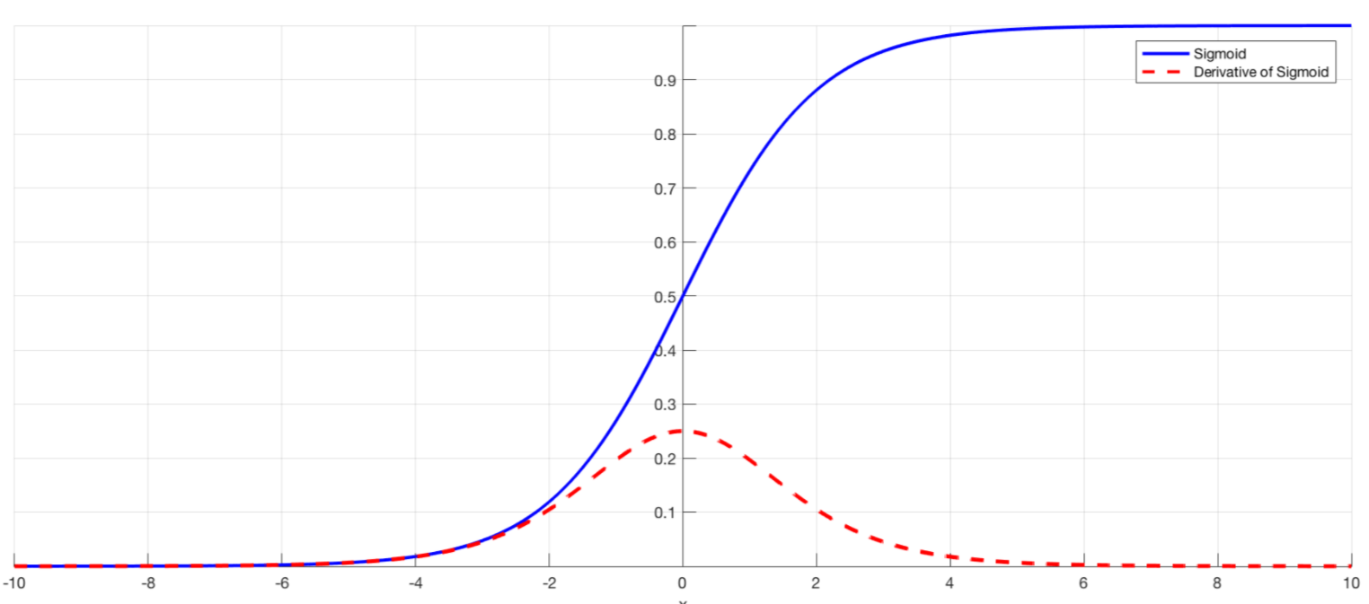
If all the weights are initialized with zero, the derivative with respect to loss function is the same for every w in W[l], thus all weights have the same value in subsequent iterations. This makes hidden units symmetric and continues for all the n iterations i.e. setting weights to zero does not make it better than a linear model. One should note that setting bias to zero will not have any effect as non-zero weights take care of breaking the symmetry and even if bias is 0, the values in every neuron will still be different.
Random Initialization: In this technique, we assign random values (expect zero) to the weights of the neural network. This technique in general helps to break the symmetry as caused in the zero initialization. It prevents neurons from learning the same features of their inputs since our goal is to make each neuron learn different functions of its input and this technique performs better than zero initialization.
As we assign random values to the weights using this technique, this may also lead to some problems:
Vanishing Gradients : If the weights initialized are very small then in case of deep networks, for any activation function, absolute value of (dW) will get smaller and smaller as we go backwards with every layer during back propagation. The earlier layers are the slowest to train in such a case. The weight update will be minor and results in slower convergence. This makes the optimization of the loss function slow. In the worst case, this may completely stop the neural network from training further.
Exploding Gradients: This is the exact opposite of the vanishing gradients problem. Consider you have non-negative and large weights and small activations A (as can be the case for sigmoid(z)). When these weights are multiplied along the layers, they cause a large change in the cost. Thus, the gradients are also going to be large. This means that the changes in W, by W — ⍺ * dW, will be in huge steps, the downward moment will increase. This may result in oscillating around the minima or even overshooting the optimum again and again and the model won’t be able to learn.
In the two procedures discussed above, we discussed the problems they can have, now we will discuss some solutions and heuristics which one can use to perform a better training of neural networks:
Using ReLu or Leaky ReLu as Activation functions:
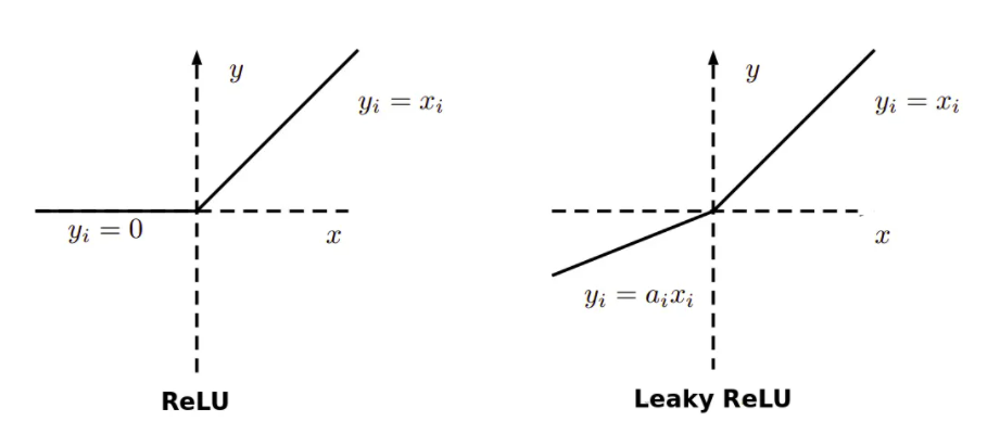
It is relatively robust to the vanishing/exploding gradient issue (especially for networks that are not too deep). With ReLu vanishing gradients are generally not a problem as the gradient is 0 for negative (and zero) inputs and 1 for positive inputs. In the case of leaky ReLu, they never have 0 gradient. Thus they never die and training continues.
Using heuristics for weight initialization:
In the previous technique using random initialization, we used to draw the numbers from standard normal distribution. Using the heuristics now, we initialize the weights depending on the non-linear activation function. Instead of drawing from standard normal distribution, we are drawing W from normal distribution with variance k/n, where k depends on the activation function. While these heuristics do not completely solve the exploding/vanishing gradients issue, they help mitigate it to a great extent.
We can use any of the following heuristics to initialize the weights depending on the chosen non-linear activation function:
For ReLu Activation: The heuristic in this case is called He Initialization, it is also called Kaiming Initialization. In this heuristic, we multiply the randomly generated values of W by:
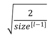
Here the value of k is 2. Here size[l-1] is the number of neurons in the previous layer (l-1).This initialization preserves the non-linearity of activation functions such as ReLu activations. Using the He method, we can reduce or magnify the magnitudes of inputs exponentially.
For Sigmoid and Tanh Activation: The heuristic in this case is called Xavier or Glorot Initialization. In this heuristic, we multiply the randomly generated values of W by:
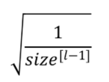
Here the value of k is 1. Xavier proposed this heuristic which is a more straightforward method, where the weights such as the variance of the activations are the same across every layer. This will prevent the gradient from exploding or vanishing.
Other similar heuristic: In this heuristic, we multiply the randomly generated values of W by:
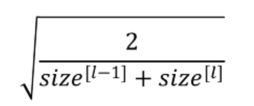
These serve as good starting points for initialization and mitigate the chances of exploding or vanishing gradients.The main objective is to minimize the variance of the parameters. They set the weights neither too much bigger than 1, nor too much less than 1. So, the gradients do not vanish or explode too quickly and it helps to avoid slow convergence, also ensuring that we do not keep oscillating off the minima.
Output:
Running the code generates the weights and prints the summary statistics.
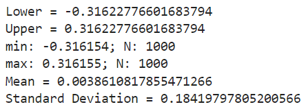
We can see that the bounds of the weight values are about -0.316 and 0.316. These bounds would become wider with fewer inputs and more narrow with more inputs. We can see that the generated weights respect these bounds and that the mean weight value is close to zero with the standard deviation close to 0.18. It can also help to see how the spread of the weights changes with the number of inputs.
To initialize the weights of your custom neural network using different methods, one can import these initializers from the following package:
org.jetbrains.kotlinx.dl.api.core.initializer