We always wonder why we have to learn and understand so many facts in math and where it gets used in real life, where we can see the implementation and examples related to the same. If you are curious enough you will find a lot of examples around you, for example look at the Fibonacci sequence the amount of similarity it consists with the world is just mind blowing. The answer behind nature’s secret code, golden ratio, and many more phenomena is Fibonacci sequence.
Fibonacci
A significant contribution to mathematics was made by Leonardo of Pisa, better known as Fibonacci. Through the centuries, his contributions to mathematics have intrigued and inspired people to explore the subject further. His name is best known for the sequence of numbers that bears his name, Fibonacci.
Fibonacci Sequence
A series of squares arranged in spiral form explains the appearance of the Fibonacci sequence, which is very beautiful and harmonious. The starting square has a side length of 1 and the square on its left has a side length of 1. Put another square on the two squares , and its side length is 2, then ,add the squares one by one, whose side length [0,1,1,2,3,5,8,13,21,34,…..,n] and so on. Every one of these numbers equals the sum of the former two numbers, and they just form the Fibonacci sequence. Many plants and animals show these numbers in their forms and designs, as well as in architecture, music, and art.
Fn
Fibonacci Number
1
0
2
1
3
1
4
2
5
3
6
5
7
8
Formula
[0,1,1,2,3,5,8,13,21,34,…..,n]
From the sequence we can observe that
\( Fn=Fn-1 + Fn-2 \) for every \( n >1\).
\( F2=F1+F0\).
\( F3=F2+F1\).
\( F4=F3+F2\) and so on.
Example
Let’s find the Fibonacci number when n=4
Solution: By using the above formula \( Fn=Fn-1 + Fn-2 \)
Take: F0=0 and F1=1
we get
F2 = F1+F0 = 1+0 = 1
F3 = F2+F1 = 1+1 = 2
F4 = F3 + F2 = 2+1 = 3
The answer is 3 when number n=4 in Fibonacci sequence
Golden Ratio
Fibonacci Sequences are closely related to Golden Ratios. According to our knowledge, the Golden Ratio value is approximately 1.618034. It is denoted by the symbol “φ”. If we take the ratio of two successive Fibonacci numbers, the ratio is close to the Golden ratio. It means that if the pair of Fibonacci numbers are of bigger value, then the ratio is very close to the Golden Ratio. So, with the help of Golden Ratio, we can find the Fibonacci numbers in the sequence. The formula is as follows \(large phi =frac{1+sqrt{5}}{2}\).
F2/F1 = 1/1 = 1
F3/F2 = 2/1 = 2
F4/F3 = 3/2 = 1.5
F5/F4 = 5/3 = 1.667
F6/F5 = 8/5 = 1.6
F7/F6 = 13/8 = 1.625
F8/F7 = 21/13 = 1.615
F9/F8 = 34/21 = 1.619
F10/F9 = 55/34 = 1.617
F11/F10 = 89/55 = 1.618
The Values of Golden Ratio is 1.618
Below is the diagrammatic representation of Fibonacci sequence
Fibonacci Sequence in Pascal’s triangle
Fibonacci numbers in Pascal’s Triangle The Fibonacci Numbers are also applied in Pascal’s Triangle. Entry is the sum of the two numbers either side of it, but in the row below. Diagonal sums in Pascal’s Triangle are the Fibonacci numbers.
In the below graph you can clearly see how the Fibonacci sequence is hidden in Pascal’s triangle.
Fibonacci sequence hidden in pascal’s triangle
Applications
Occurrence of Fibonacci Sequence can be seen and found almost everywhere within our universe. Below are some examples where it can be seen.
Petals of flowers is where it covers most of its’ property.
1 petal: white calla lily
3 petals: iris
5 petals: buttercup
8 petals: delphiniums
13 petals: cineraria
used in the grouping of numbers and the brilliant proportion in music generally.
used in Coding (computer algorithms, interconnecting parallel, and distributed systems)
in numerous fields of science including high-energy physical science, quantum mechanics, Cryptography, etc.
Mind Blowing Properties
There are too many properties some of them are mentioned below:
Summing together any ten consecutive Fibonacci numbers will always result in a number which is divisible by eleven
Any two consecutive Fibonacci numbers are relatively prime, having no factors in common with each other
Every third Fibonacci number is divisible by two,
Every fourth Fibonacci number is divisible by three, or . Every fifth Fibonacci number is divisible by five and pattern continues
If any two consecutive Fibonacci numbers are squared and then added together, the result is a Fibonacci number, which will form a sequence of alternate Fibonacci numbers.
Let’s Jump to Code
val Input = 15
   println("The number is defined as: $Input")
   fibonacciSeries(Input)
fun fibonacciSeries(Input: Int) {
   var temp1 = 0
   var temp2 = 1
   println("The fibonacci series till $Input terms:")
   for (i in 1..Input) {
      print("$temp1 ")
      val sum = temp1 + temp2
      temp1 = temp2
      temp2 = sum
   }
}
Output
The number is defined as: 15
The Fibonacci series till 15 terms:
0 1 1 2 3 5 8 13 21 34 55 89 144 233 377
Conclusion
I think the Fibonacci sequence is the only pattern whose existence is too fascinating. Other than this I don’t think there is something of this magnitude present in our universe. It is a great example of how vast and interesting and fun math is which literally makes us believe that everything is possible when you have the vision of math.
An object’s acceleration is the rate at which its velocity changes over time. The acceleration of an object is the result of all the forces acting on it, according to Newton’s second law. Gravity is the only force acting on a freely falling object under ideal circumstances. Calculate the displacement of an object that is free falling, calculate its average velocity at set intervals, and calculate its acceleration due to gravity.
Theory
When do we get to know if there is acceleration or not?
Drop something you pick up with your hand. As soon as you release it from your hand, its speed is zero. As it descends, its speed increases. As it falls, it travels faster. To me, that sounds like acceleration.
Acceleration is not just about increasing speed. Toss this same object vertically into the air. On the way up, its speed decreases until it stops and reverses direction. Acceleration also refers to a decrease in speed.
Acceleration involves more than just changing speed. One last time, launch your battered object. Throw it horizontally this time, and observe how its horizontal velocity gradually becomes vertical. Considering that acceleration is the rate at which velocity changes with time and velocity is a vector quantity, this change in direction is also considered acceleration.
Gravity was pulling the object down, so it was accelerating. The moment an object leaves your hand, it begins to fall – even if thrown straight up. In the absence of this, it would have continued moving away from you in a straight line. Gravity causes this acceleration.
Gravitational acceleration varies slightly with latitude and height above the earth’s surface. Sea level is experiencing greater acceleration due to gravity than Mount Everest at sea level and the poles are experiencing greater acceleration due to gravity at the equator. Free falling objects do not encounter a significant amount of air resistance; they fall solely under the influence of gravity. No matter how heavy an object is, it will fall with the same rate of acceleration. Galileo demonstrated with a demonstration that mass doesn’t really matter when it comes to free falling, contrary to what was previously thought.
Famous leaning tower of Pisa demonstration
This phenomenon was also observed by Galileo, who recognized that it was contrary to Aristotle’s principle that heavier items fall more quickly. According to an apocryphal tale, Galileo (or an assistant, more likely) dropped two objects of unequal mass from the Leaning Tower of Pisa. Contrary to Aristotle’s teachings, both objects struck the ground simultaneously (or very nearly so). Galileo probably couldn’t have obtained much information from this experiment given the speed at which the fall would occur. The majority of his observations of falling bodies were of round objects rolling down ramps. Water clocks and his own pulse were used to measure the time intervals (stopwatches and photogates hadn’t yet been invented). Until he reached an accuracy of one tenth of a pulse beat between two observations, he repeated this “a hundred times.”
The instant when the balls are released is considered to be the initial time t = 0. The position of the ball along the ruler is described by the variable y. The position of the ball at a time t is given by
\(\large y(t)=y_0{}+v_0t+\frac{1}{2}g t^{2}\).
If the ball is released from rest, the initial velocity is zero: v0 = 0. Therefore,
\(\large y(t)=y_0+\frac{1}{2}g t^{2}\).
Free fall bodies accelerate at -9.8 m/s (negative sign indicates downward acceleration). However, the acceleration of
A free falling body has a velocity of -9.8 m/s in the kinematic equation.
2) A drop from a particular height has an initial velocity of 0 m/s.
When an object is projected upwards vertically, it will slowly rise up. When it reaches 0 m/s, its velocity is zero
The apex of its trajectory.
Question:
Calculate the body height if it has a mass of 1 kg and after 9 seconds it reaches the ground?
Answer:
Given: Height h =? Time t = 9s We all are acquainted with the fact that free fall is independent of mass.
Hence, it is given as
\(\large h=\frac{1}{2}g t^{2}\).
h=0.5 * 9.8 * (9)2
h= 396.9
Falling with Air Resistance
It is common for an object to encounter some degree of air resistance as it falls through the air. Air molecules collide with the object’s leading surface, causing air resistance. There are a variety of factors that determine how much air resistance the object encounters. The speed of the object and its cross-sectional area are two factors that have a direct effect upon the amount of air resistance. An increase in speed results in an increase in air resistance. The amount of air resistance increases with an increase in cross-sectional area.
Common mistakes and misconceptions
A falling object’s final velocity is mistakenly assumed to be zero once it hits the ground. It is the speed just before touching the ground that determines the final velocity in physics problems. As soon as the object touches the ground, it ceases to be in freefall.
Math Coding
    fun height(gravity: Double, seconds: Double): Double {
        return 0.5 * gravity * Math.pow(seconds, 2.0)
    }

    fun velocity(gravity: Double, seconds: Double): Double {
        return gravity * seconds
    }

    fun time(velocity: Double, gravity: Double): Double {
        return velocity / gravity
    }

    //Execution for Test Purpose
        val gravity = 9.80665
        var time = 10.0
        val height = height(gravity, time)
        val velocity = velocity(gravity, time)
        time = time(velocity, gravity)
        println("$velocity m/s")
        println("$time seconds")
        println("$height meter")
Output
98.06649999999999 m/s
10.0 seconds
490.3325 meter
Conclusion
A free-falling object is studied using the kinematic equations. As a free falling object falls, it will be influenced by gravity. A free falling object has two main characteristics: it does not encounter air resistance, and it accelerates at a rate of 9.8 m/2. We can determine the height, velocity and time of free fall using the formula.
Let us assume we have to find the answer to a question which is something like this: A car starts from rest and covers some distance in some seconds with constant acceleration. Find the acceleration of the car. In this scenario you have to deal with the speed of the car, distance, time taken, displacement, etc. equation of motion is required.
Classical mechanics is based on the Equations of Motion. For all macroscopic bodies moving at a speed considerably less than the speed of light, analysis of motion is done using Newton’s Equations of Motion. In this article, we will learn about these laws and their derivations along with the code in Kotlin S2.
Motion
First of all, let us know what motion actually is. As derived by the famous scientist Sir Isaac Newton we can define that motion as change in the position of an object with respect to time. That is, how much the object has moved in a time interval. We can represent the position using a reference point and then we can calculate the distance travelled by the object from that reference point. Similarly, we can calculate the time using a speed-watch which will represent the time taken for the change to happen.
Descriptions of motion
\(d\) is the distance.
\(s\) is displacement.
\(u\) is initial velocity.
\(v\) is final velocity.
\(a\) is acceleration.
\(t\) is the time taken for the motion to happen.
Distance
Distance is the actual measure of an object’s total change in position (over a period of time).
Note: Since distance is a scalar quantity hence it represents only the magnitude or the size or “how much”.
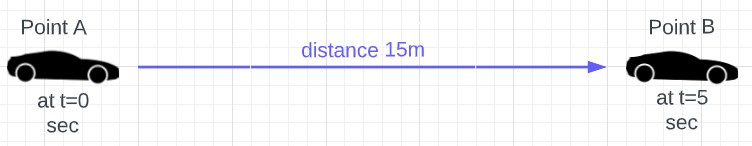
Displacement
Displacement is defined as change in the position of an object(car). The arrow from point A to point B represents the change in the initial and final position of the object(car).
Note: Unlike distance, displacement is a vector quantity (an arrow) hence it represents both magnitude and direction, i.e., how much and which way.
Speed
Speed is a measure of how fast or slow an object(car) moves or changes its position. Speed is equal to the change in the distance covered by the object(car) per each unit of time. Mathematically speed is the ratio between the distance and time, i.e., distance divided by time.
\(v=\frac{\text{distance}}{\text{time}}\) i.e. \(v=\frac{d}{t}\)
The above graph gives us information about distance and time. By using the formula, we can calculate the speed. Let’s do it.
Question: If a car has traveled a total distance of 15m in 5 sec. calculate the speed.
Note: Speed is also a scalar quantity since both time and distance are scalar quantities too.
Velocity
Velocity can be defined as the rate of change of displacement of an object(car) per time unit, e.g., each second, each hour or each day. Mathematically this rate of change of position can represent as
By looking at the above figure we get to know a couple of things like distance, displacement and time so by using the above formula we can easily calculate the velocity.
Question: If a car has covered 20m distance in 3 sec, calculate the velocity.
Note: Velocity is vector quantity. It has information about both magnitude/size and direction.
Acceleration
Acceleration is the rate of change of the velocity of an object with respect to time. It is how much the velocity changes in a time unit. Acceleration is also a vector quantity and mathematically we can represent it as:
If the acceleration is negative, the object is slowing down. If the acceleration is positive, the object is speeding up. Watch out for the traffic police!
Equations of motion
The nature and the behavior of a physics system in terms of motion is determined by the equations of motion. There are three equations of motion.
\(v=u+at\),
\(s=u t+\frac{1}{2}at^{2}\),
\(v^{2}=u^{2}+2as\).
Derivation of the Equations of Motion by the Algebraic Method
Let’s see the derivations of the equations of motion by the algebraic method.
1st Equation of Motion
We all know that in general, acceleration is defined as the rate at which a body’s velocity changes over time. That is, how much the velocity changes in each unit of time. Mathematically, it is the difference in the final and initial velocities divided by the time taken for the change to happen.
\(\text{acceleration}(a)=\frac{(v-u)}{t}\).
where,
\(u\) = initial velocity
\(v\) = final velocity,
\(t\) = time taken
When we rearrange the above equation we get the following 1st equation of motion.
\(v=u+at\)
2nd Equation of Motion
Imagine a body moving with an initial velocity of \(u\) under constant acceleration \(a\). The speed of the body becomes \(v\) after time \(t\) and the displacement becomes \(s\).
The velocity of an object is defined as the rate at which its displacement changes, or alternatively the displacement changes per unit of time. We can represent this mathematically as:
If the velocity is not constant then we can use the average velocity in the place of velocity in the above equation, and rewrite the equation as follows:
Now, from the 1st equation of motion, we know that
\(v=u + at\).
Rearranging the above formula,
we get
\(t = \frac{u-v}{a}\).
Now, substituting this value of \(t\) in the displacement formula we get the following equations.
\(s = \frac{(u+v)}{2} * \frac{v-u}{a}\),
\(2as=v^{2}-u^{2}\),
\(v^{2}=u^{2}+2as\).
Derivation of the Equations of Motion by the Calculus Method
Let’s demonstrate the derivations of the Equation of Motion by using the Calculus Method.
1st Equation of Motion
The acceleration of the object is constant so we use the definition of the instantaneous acceleration of the particle. That is, the acceleration of the object at a time point (rather than a time interval).
Here, initial velocity = \(u\), the final velocity = \(v\), and the time interval \(dt\) is taken from \(t = o\) to \(t\) second.
The change in velocity \(dv\) is therefore the sum of all instantaneous acceleration \(a\) over all time points \(dt\). When \(a\) is a constant, it is simply
After rearranging we get the 3rd equation of motion.
\(v^{2} = u^{2} + 2as\).
Math Coding
Enough of theory, let’s now jump to some hands-on experiment with what we just learned. We will do the math coding of the equations of motion in S2.
// 1st equation of motion: final velocity
fun v(u : Double, a : Double, t : Double) : Double {
    var v = u + a * t;
    return v;
}

// compute the final velocity with inputs
// initial velocity = 5.0 m/s, acceleration = 2.0 m/s/s, time = 10 sec
val v = v(5.0, 2.0, 10.0)

// print out the final velocity
v
Here we set the initial velocity \(u = 5.0\) meters per second, acceleration \(a = 2.0\) meters per second per second and time \(t = 10.0\) seconds. The output is as follows:
25.0
We use two different ways to compute the displacement. We first use the second equation.
// 2nd equation of motion: displacement
fun s_1(u : Double, a : Double, t : Double) : Double {
    var s = u * t + 0.5 * a * t * t;
    return s;
}

// compute the displacement
// initial velocity = 5.0 m/s, acceleration = 2.0 m/s/s, time = 10 sec
val s_1 = s_1(5.0, 2.0, 10.0)

// print out the displacement
s_1
The output is as follows.
150.0
Alternatively, we can compute the displacement using the third equation of motion.
// 3rd equation of motion: displacement
// another formula to compute displacement
fun s_2(u : Double, a : Double, t : Double) : Double {
    var s = (v*v - u*u) / 2.0 / a;
    return s;
}

// compute the displacement
// initial velocity = 5.0 m/s, acceleration = 2.0 m/s/s, time = 10 sec
val s_2 = s_2(5.0, 2.0, 10.0)

// print out the displacement
s_2
The output is as follows.
150.0
We can also use the third equation of motion to compute the final velocity. We need to compute the square of velocity first.
// 3rd equation of motion: velocity squared
fun v2(u : Double, a : Double, s : Double) : Double {
    var v2 = u*u + 2.0 * a * s;
    return v2;
}

// compute the square of the final velocity
// initial velocity = 5.0 m/s, acceleration = 2.0 m/s/s, displacement = 150 m
val v2 = v2(5.0, 2.0, 150.0)

// print out the velocity squared
v2
The output is as follows.
625.0
The final velocity is the square root of the last result.
// print out the final velocity
sqrt(v2)
25.0
As expected, it is the same as what we input for the first two equations.
Try out the equations with your own input and numbers. Play with the code to see what you get. It is fun to do experiments! Let us what you think and leave us comments below.
It is important to note that we have derived the set of equations of motion without doing experiments or data. We construct a theory entirely out of imagination. The concept of space (position) and time are intuitive. We can measure them using a ruler and a clock. While the concept of speed may be familiar by daily experience, the concept of acceleration is a pure theoretical construct. By introducing or inventing the “new” notion of acceleration, we construct a theory of motion, and tie together all fundamental quantities, namely, space, time, and velocity, using precise mathematical equations. This illustrates how we can invent new physics theory using pure imagination. This is true for our simple framework of motion but it is also true for much more advanced theories like the Special Relativity. Both Newton and Einstein constructed their ground breaking theories by inventing new concepts by pure imagination without actually doing any experiments or data. They then expressed their concepts precisely using mathematics.